Eigendecomposition for 2D Whittaker Baselines

This example will examine using eigendecomposition to solve Whittaker-smoothing-based baselines for two dimensional data.

As explained in the 2D Algorithms section, solving the analytical solution for Whittaker-smoothing-based algorithms is computationally demanding. Through the use of eigendecomposition, the effective dimension of the system can be reduced and allow solving much faster. The number of eigenvalues required to represent the baseline depends on the curvature of the baseline, so this example will examine a low order polynomial baseline and a sinusoidal baseline, which represent low and high curvature, respectively.

from time import perf_counter

import matplotlib.pyplot as plt
import numpy as np

from pybaselines import Baseline2D
from pybaselines.utils import gaussian2d


def mean_squared_error(fit_baseline, real_baseline):
    """Calculate the mean-squared error compared to the true baseline."""
    return ((fit_baseline - real_baseline)**2).mean()


def plot_contour_with_projection(X, Z, data, title=''):
    """Plots the countour plot and 3d projection."""
    fig = plt.figure(layout='constrained', figsize=plt.figaspect(0.5))
    fig.suptitle(title)
    ax_1 = fig.add_subplot(1, 2, 1, projection='3d')
    ax_1.plot_surface(X, Z, data, cmap='coolwarm')
    ax_2 = fig.add_subplot(1, 2, 2)
    ax_2.contourf(X, Z, data, cmap='coolwarm')


x = np.linspace(-20, 20, 100)
z = np.linspace(-20, 30, 100)
X, Z = np.meshgrid(x, z, indexing='ij')
signal = (
    gaussian2d(X, Z, 12, -5, -5)
    + gaussian2d(X, Z, 11, 3, 2)
    + gaussian2d(X, Z, 13, 8, 8)
    + gaussian2d(X, Z, 8, 9, 18)
    + gaussian2d(X, Z, 16, -8, 8)
)
polynomial_baseline = 0.1 + 0.05 * X + 0.005 * Z - 0.008 * X * Z + 0.0006 * X**2 + 0.0003 * Z**2
sine_baseline = np.sin(X / 5) + np.cos(Z / 2)
noise = np.random.default_rng(0).normal(scale=0.1, size=signal.shape)
y = signal + noise + polynomial_baseline
y2 = signal + noise + sine_baseline

Only the baselines will be plotted in this example since the actual data is irrelevant for this discussion.

plot_contour_with_projection(X, Z, polynomial_baseline, title='Actual Polynomial Baseline')
plot_contour_with_projection(X, Z, sine_baseline, title='Actual Sinusoidal Baseline')

• 
• 

The lam values for fitting the baseline can be kept constant whether using eigendecomposition or the analytical solution.

lam_poly = (1e2, 1e4)
lam_sine = (1e2, 1e0)
baseline_fitter = Baseline2D(x, z)

t0 = perf_counter()
analytical_poly_baseline, params_1 = baseline_fitter.arpls(y, lam=lam_poly, num_eigens=None)
analytical_sine_baseline, params_2 = baseline_fitter.arpls(y2, lam=lam_sine, num_eigens=None)
t1 = perf_counter()
mse_analytical_poly = mean_squared_error(analytical_poly_baseline, polynomial_baseline)
mse_analytical_sine = mean_squared_error(analytical_sine_baseline, sine_baseline)
print(f'Analytical solutions:\nTime: {t1 - t0:.3f} seconds')
print(f'Mean-squared-error, polynomial: {mse_analytical_poly:.5f}')
print(f'Mean-squared-error, sinusoidal: {mse_analytical_sine:.5f}\n')

plot_contour_with_projection(
    X, Z, analytical_poly_baseline, title='Analytical Polynomial Baseline'
)
plot_contour_with_projection(
    X, Z, analytical_sine_baseline, title='Analytical Sinusoidal Baseline'
)

• 
• 

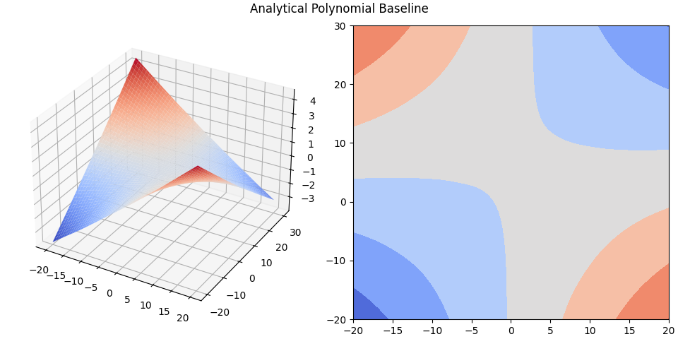
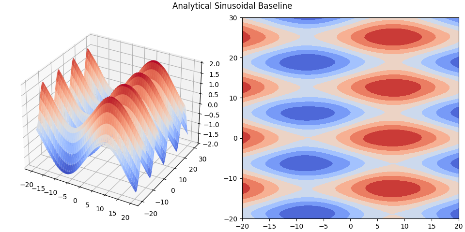
Analytical solutions:
Time: 4.340 seconds
Mean-squared-error, polynomial: 0.00014
Mean-squared-error, sinusoidal: 0.00099

Now, try using eigendecomposition to calculate the same baselines. To start off, 40 eigenvalues will be used along the rows and columns. Note that return_dof is set to True so that the effective degrees of freedom for each eigenvector is calculated and returned in the parameters dictionary. This allows plotting the degrees of freedom for determining how many eigenvalues are actually needed.

num_eigens = (40, 40)

t0 = perf_counter()
eigenvalue_poly_baseline_1, params_3 = baseline_fitter.arpls(
    y, lam=lam_poly, num_eigens=num_eigens, return_dof=True
)
eigenvalue_sine_baseline_1, params_4 = baseline_fitter.arpls(
    y2, lam=lam_sine, num_eigens=num_eigens, return_dof=True
)
t1 = perf_counter()
mse_analytical_poly = mean_squared_error(eigenvalue_poly_baseline_1, polynomial_baseline)
mse_analytical_sine = mean_squared_error(eigenvalue_sine_baseline_1, sine_baseline)
print(f'40x40 Eigenvalues:\nTime: {t1 - t0:.3f} seconds')
print(f'Mean-squared-error, polynomial: {mse_analytical_poly:.5f}')
print(f'Mean-squared-error, sinusoidal: {mse_analytical_sine:.5f}\n')

plot_contour_with_projection(
    X, Z, eigenvalue_poly_baseline_1, title='40x40 Eigenvalues Polynomial Baseline'
)
plot_contour_with_projection(
    X, Z, eigenvalue_sine_baseline_1, title='40x40 Eigenvalues Sinusoidal Baseline'
)

• 
• 

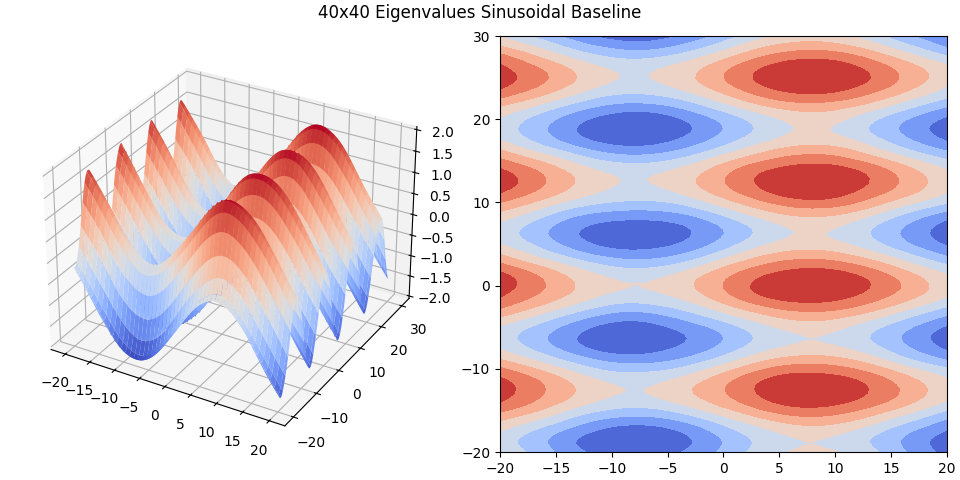
40x40 Eigenvalues:
Time: 9.635 seconds
Mean-squared-error, polynomial: 0.00014
Mean-squared-error, sinusoidal: 0.00100

By using 40 eigenvalues along the rows and 40 along the columns, the error of the fit remains the same as the analytical solution while slightly reducing the computation time. However, the number of eigenvalues being used is more than is actually required to represent the two baselines, which means that the calculation time can be further reduced. Plot the effective degrees of freedom to see which contribute most to the calculation.

plot_contour_with_projection(
    *np.meshgrid(np.arange(num_eigens[0]), np.arange(num_eigens[1]), indexing='ij'),
    params_3['dof'], title='Effective Degrees of Freedom for Polynomial Baseline'
)
plot_contour_with_projection(
    *np.meshgrid(np.arange(num_eigens[0]), np.arange(num_eigens[1]), indexing='ij'),
    params_4['dof'], title='Effective Degrees of Freedom for Sinusoidal Baseline'
)

• 
• 

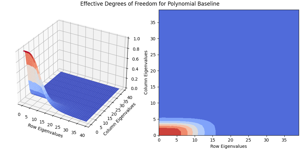
A very rough rule of thumb for determining the number of eigenvalues required is to select where the second derivative of the effective degrees of freedom reaches 0 (note that this is not based off of any math, just from testing various baselines). For the polynomial baseline, this is at about 10 eigenvalues for the rows and 4 for the columns. For the sinusoidal baseline, this is at approximately 8 eigenvalues for the rows and 35 for the columns. Now, let's see if reducing the number of eigenvalues improves the calculation time without increasing the error.

num_eigens_poly = (10, 4)
num_eigens_sine = (8, 35)

t0 = perf_counter()
eigenvalue_poly_baseline_2, params_5 = baseline_fitter.arpls(
    y, lam=lam_poly, num_eigens=num_eigens_poly, return_dof=True
)
eigenvalue_sine_baseline_2, params_6 = baseline_fitter.arpls(
    y2, lam=lam_sine, num_eigens=num_eigens_sine, return_dof=True
)
t1 = perf_counter()
mse_analytical_poly = mean_squared_error(eigenvalue_poly_baseline_2, polynomial_baseline)
mse_analytical_sine = mean_squared_error(eigenvalue_sine_baseline_2, sine_baseline)
print(f'10x4 Eigenvalues for polynomial, 8x35 for sinusoidal:\nTime: {t1 - t0:.3f} seconds')
print(f'Mean-squared-error, polynomial: {mse_analytical_poly:.5f}')
print(f'Mean-squared-error, sinusoidal: {mse_analytical_sine:.5f}\n')

plot_contour_with_projection(
    X, Z, eigenvalue_poly_baseline_2, title='10x4 Eigenvalues Polynomial Baseline'
)
plot_contour_with_projection(
    X, Z, eigenvalue_sine_baseline_2, title='8x35 Eigenvalues Sinusoidal Baseline'
)

• 
• 

10x4 Eigenvalues for polynomial, 8x35 for sinusoidal:
Time: 0.376 seconds
Mean-squared-error, polynomial: 0.00015
Mean-squared-error, sinusoidal: 0.00070

By reducing the number of eigenvalues to represent the baseline, the calculation time is reduced by about an order of magnitude, and the error of the two calculations does not significantly change, showing the efficacy of this approach.

Finally, let's see the effects of using significantly less eigenvalues than are needed.

num_eigens_poly = (3, 3)
num_eigens_sine = (5, 12)

t0 = perf_counter()
eigenvalue_poly_baseline_3, params_7 = baseline_fitter.arpls(
    y, lam=lam_poly, num_eigens=num_eigens_poly, return_dof=True
)
eigenvalue_sine_baseline_3, params_8 = baseline_fitter.arpls(
    y2, lam=lam_sine, num_eigens=num_eigens_sine, return_dof=True
)
t1 = perf_counter()
mse_analytical_poly = mean_squared_error(eigenvalue_poly_baseline_3, polynomial_baseline)
mse_analytical_sine = mean_squared_error(eigenvalue_sine_baseline_3, sine_baseline)
print(f'3x3 Eigenvalues for polynomial, 5x12 for sinusoidal:\nTime: {t1 - t0:.3f} seconds')
print(f'Mean-squared-error, polynomial: {mse_analytical_poly:.5f}')
print(f'Mean-squared-error, sinusoidal: {mse_analytical_sine:.5f}')

plot_contour_with_projection(
    X, Z, eigenvalue_poly_baseline_3, title='3x3 Eigenvalues Polynomial Baseline'
)
plot_contour_with_projection(
    X, Z, eigenvalue_sine_baseline_3, title='5x12 Eigenvalues Sinusoidal Baseline'
)

plt.show()

• 
• 

3x3 Eigenvalues for polynomial, 5x12 for sinusoidal:
Time: 0.138 seconds
Mean-squared-error, polynomial: 0.00015
Mean-squared-error, sinusoidal: 0.02029

While the error for the polynomial baseline does not increase significantly, the error for the sinusoidal baseline fit does since there are too few eigenvalues now to represent the total required curvature.