Morphological Baselines
Introduction
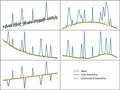
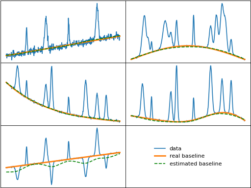
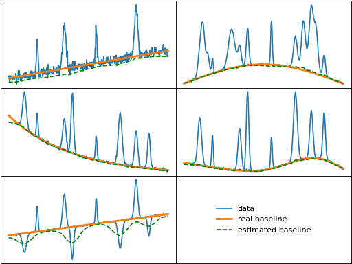
Morphological operations include dilation, erosion, opening, and closing, and they use moving windows to compute the maximum, minimum, or a combination of the two within each window, as shown in the figures below. The algorithms in this section use these operations to estimate the baseline.

Note
All morphological algorithms use a half_window parameter to define the size
of the window used for the morphological operators. half_window is index-based,
rather than based on the units of the data, so proper conversions must be done
by the user to get the desired window size.
Algorithms
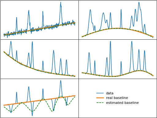
mpls (Morphological Penalized Least Squares)
mpls() uses both morphological operations and Whittaker-smoothing
to create the baseline. First, a morphological opening is performed on the
data. Then, the index of the minimum data value between each flat region of the
opened data is selected as a baseline anchor point and given a weighting of
\(1 - p\), while all other points are given a weight of \(p\). The data
and weights are then used to calculate the baseline, similar to the asls()
method.
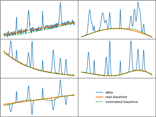
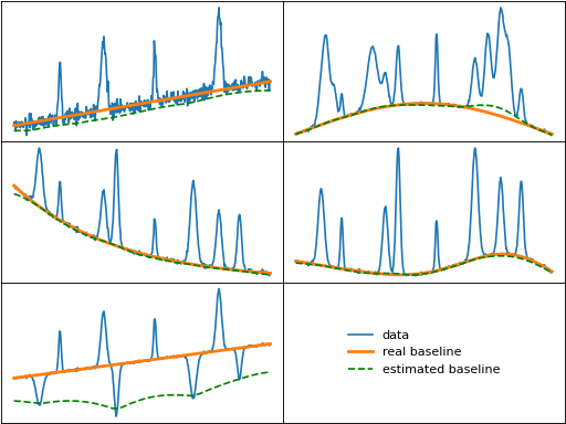
mor (Morphological)
mor() performs a morphological opening on the data and then selects
the element-wise minimum between the opening and the average of a morphological
erosion and dilation of the opening to create the baseline.
Note
The baseline from the mor method is not smooth. Smoothing is left to the user to perform, if desired.
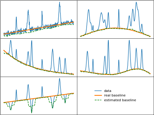
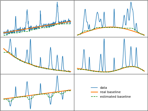
imor (Improved Morphological)
imor() is an attempt to improve the mor method, and iteratively selects the element-wise
minimum between the original data and the average of a morphological erosion and dilation
of the opening of either the data (first iteration) or previous iteration's baseline to
create the baseline.
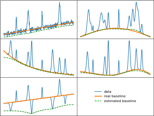
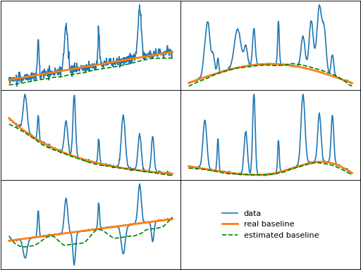
mormol (Morphological and Mollified Baseline)
mormol() iteratively convolves the erosion of the data with a mollifying (smoothing)
kernel, to produce a smooth baseline.
amormol (Averaging Morphological and Mollified Baseline)
amormol() iteratively convolves a mollifying (smoothing) kernel with the
element-wise minimum of the data and the average of the morphological closing
and opening of either the data (first iteration) or previous iteration's baseline.
rolling_ball (Rolling Ball)
rolling_ball() performs a morphological opening on the data and
then smooths the result with a moving average, giving a baseline that
resembles rolling a ball across the data.
mwmv (Moving Window Minimum Value)
mwmv() performs a morphological erosion on the data and
then smooths the result with a moving average.
tophat (Top-hat Transformation)
tophat() performs a morphological opening on the data.
Note
The baseline from the tophat method is not smooth. Smoothing is left to the user to perform, if desired.
mpspline (Morphology-Based Penalized Spline)
mpspline() uses both morphological operations and penalized splines
to create the baseline. First, the data is smoothed by fitting a penalized
spline to the closing of the data with a window of 3. Then baseline points are
identified where the smoothed data is equal to the element-wise minimum between the
opening of the smoothed data and the average of a morphological erosion and dilation
of the opening. The baseline points are given a weighting of \(1 - p\), while all
other points are given a weight of \(p\), similar to the mpls() method.
Finally, a penalized spline is fit to the smoothed data with the assigned weighting.
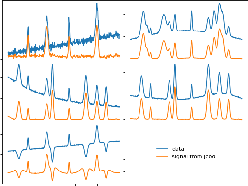
jbcd (Joint Baseline Correction and Denoising)
jbcd() uses regularized least-squares fitting combined with morphological operations
to simultaneously obtain the baseline and denoised signal.
Minimized function:
where \(y_i\) is the measured data, \(v_i\) is the estimated baseline, \(s_i\) is the estimated signal, \(\Delta^d\) is the forward-difference operator of order d, \(Op_i\) is the morphological opening of the measured data, and \(\alpha\), \(\beta\), and \(\gamma\) are regularization parameters.
Linear systems:
The initial signal, \(s^0\), and baseline, \(v^0\), are set equal to \(y\), and \(Op\), respectively. Then the signal and baseline at iteration \(n\), \(s^n\) and \(v^n\), are solved for sequentially using the following two linear equations:
where \(I\) is the identity matrix and \(D_d\) is the matrix version of \(\Delta^d\), which is also the d-th derivative of the identity matrix. After each iteration, \(\beta\), and \(\gamma\) are updated by user-specified multipliers.
The signal with the baseline removed and noise decreased can also be obtained from the output of the jbcd function.