Classification Baselines

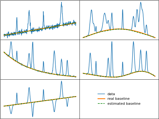
The contents of pybaselines.classification contain algorithms that rely on classifying peak and/or baseline segments.

Introduction

Classification methods are similar to selective masking as explained in the polynomial section, but use sophisticated techniques to determine the baseline points rather than relying on manual selection.

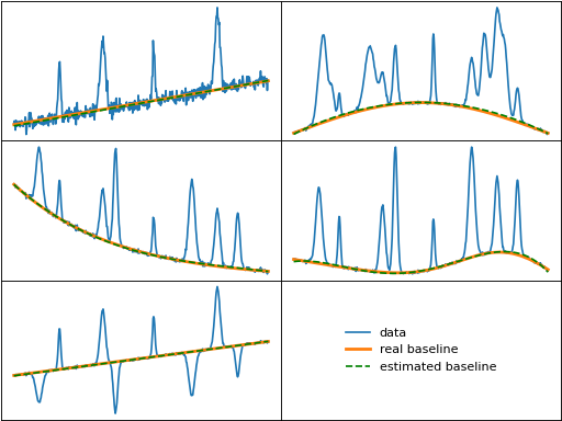
All classification functions allow inputting weights to override the baseline classification, which can be helpful, for example, to ensure a small peak is not classified as baseline without having to alter any parameters which could otherwise reduce the effectiveness of the classification method. The plot below shows such an example.

(Source code, png)

Algorithms

dietrich (Dietrich's Classification Method)

dietrich() calculates the power spectrum of the data as the squared derivative of the data. Then baseline points are identified by iteratively removing points where the mean of the power spectrum is less a multiple of the standard deviation of the power spectrum. The baseline is created by first interpolating through all baseline points, and then iteratively fitting a polynomial to the interpolated baseline.

(Source code, png)

golotvin (Golotvin's Classification Method)

golotvin() divides the data into sections and takes the minimum standard deviation of all the sections as the noise's standard deviation for the entire data. Then classifies any point where the rolling max minus min is less than a multiple of the noise's standard deviation as belonging to the baseline.

(Source code, png)

std_distribution (Standard Deviation Distribution)

std_distribution() identifies baseline segments by analyzing the rolling standard deviation distribution. The rolling standard deviations are split into two distributions, with the smaller distribution assigned to noise. Baseline points are then identified as any point where the rolled standard deviation is less than a multiple of the median of the noise's standard deviation distribution.

(Source code, png)

fastchrom (FastChrom's Baseline Method)

fastchrom() identifies baseline segments by analyzing the rolling standard deviation distribution, similar to std_distribution(). Baseline points are identified as any point where the rolling standard deviation is less than the specified threshold, and peak regions are iteratively interpolated until the baseline is below the data.

(Source code, png)

cwt_br (Continuous Wavelet Transform Baseline Recognition)

cwt_br() identifies baseline segments by performing a continous wavelet transform (CWT) on the input data at various scales, and picks the scale with the first local minimum in the Shannon entropy. The threshold for baseline points is obtained by fitting a Gaussian to the histogram of the CWT at the optimal scale, and the final baseline is fit using a weighted polynomial where identified baseline points are given a weight of 1 while all other points have a weight of 0.

(Source code, png)

fabc (Fully Automatic Baseline Correction)

fabc() identifies baseline segments by thresholding the squared first derivative of the data, similar to dietrich(). However, fabc approximates the first derivative using a continous wavelet transform with the Haar wavelet, which is more robust to noise than the numerical derivative in Dietrich's method. The baseline is then fit using Whittaker smoothing with all baseline points having a weight of 1 and all other points a weight of 0.

(Source code, png)

rubberband (Rubberband Method)

rubberband() uses a convex hull to find local minima of the data, which are then used to construct the baseline using either linear interpolation or Whittaker smoothing. The rubberband method is simple and easy to use for convex shaped data, but performs poorly for concave data. To get around this, Bruker's OPUS spectroscopy software uses a patented method to coerce the data into a convex shape so that the rubberband method still works. pybaselines uses an alternate approach of allowing splitting the data in segments, in order to reduce the concavity of each individual section; it is less user-friendly than Bruker's method but works well enough for data with similar baselines and peak positions.

Note

For noisy data, rubberband performs significantly better when smoothing the data beforehand.

(Source code, png)

By using Whittaker smoothing (or other smoothing interpolation methods) rather than linear interpolation to construct the baseline from the convex hull points, the negative effects of applying the rubberband method to concave data can be slightly reduced, as seen below.

(Source code, png)