Whittaker Baselines

The contents of pybaselines.whittaker contain Whittaker-smoothing-based algorithms for fitting the baseline. Note that Whittaker smoothing is often also referred to as Whittaker-Henderson smoothing.

Introduction

Whittaker-smoothing-based algorithms are usually referred to in literature as weighted least squares, penalized least squares, or asymmetric least squares, but are referred to as Whittaker-smoothing-based in pybaselines to distinguish them from polynomial techniques that also take advantage of weighted least squares (like loess()) and penalized least squares (like penalized_poly()).

A great introduction to Whittaker smoothing is Paul Eilers's A Perfect Smoother paper. The general idea behind Whittaker smoothing algorithms is to make the baseline match the measured data as well as it can while also penalizing the roughness of the baseline. The resulting general function that is minimized to determine the baseline is then

\[\sum\limits_{i}^N w_i (y_i - z_i)^2 + \lambda \sum\limits_{i}^{N - d} (\Delta^d z_i)^2\]

where \(y_i\) is the measured data, \(z_i\) is the estimated baseline, \(\lambda\) is the penalty scale factor, \(w_i\) is the weighting, and \(\Delta^d\) is the finite-difference operator of order d.

The resulting linear equation for solving the above minimization is:

\[(W + \lambda D_d^{\top} D_d) z = W y\]

where \(W\) is the diagaonal matrix of the weights, and \(D_d\) is the matrix version of \(\Delta^d\), which is also the d-th derivative of the identity matrix. For example, for an array of length 5, \(D_1\) (first order difference matrix) is:

\[\begin{split}\begin{bmatrix} -1 & 1 & 0 & 0 & 0 \\ 0 & -1 & 1 & 0 & 0 \\ 0 & 0 & -1 & 1 & 0 \\ 0 & 0 & 0 & -1 & 1 \\ \end{bmatrix}\end{split}\]

and \(D_2\) (second order difference matrix) is:

\[\begin{split}\begin{bmatrix} 1 & -2 & 1 & 0 & 0 \\ 0 & 1 & -2 & 1 & 0 \\ 0 & 0 & 1 & -2 & 1 \\ \end{bmatrix}\end{split}\]

Most Whittaker-smoothing-based techniques recommend using the second order difference matrix, although some techniques use both the first and second order difference matrices.

The baseline is iteratively calculated using the linear system above by solving for the baseline, \(z\), updating the weights, solving for the baseline using the new weights, and repeating until some exit criteria. The difference between Whittaker-smoothing-based algorithms is the selection of weights and/or the function that is minimized.

Note

The \(\lambda\) (lam) value required to fit a particular baseline for all Whittaker-smoothing-based methods will increase as the number of data points increases, with the relationship being roughly \(\log(\lambda) \propto \log(\text{number of data points})\). For example, a lam value of \(10^3\) that fits a dataset with 100 points may have to be \(10^7\) to fit the same data with 1000 points, and \(10^{11}\) for 10000 points.

Algorithms

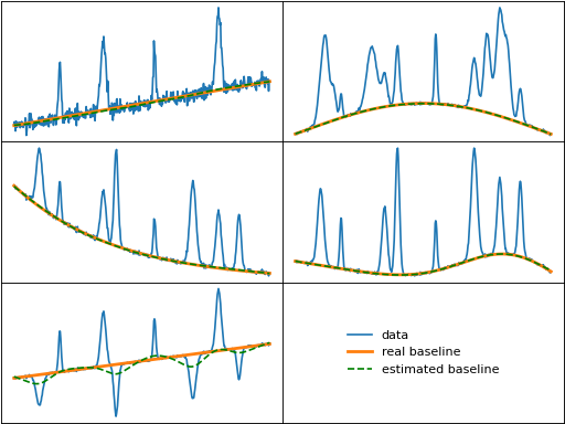
asls (Asymmetric Least Squares)

The asls() (sometimes called "ALS" in literature) function is the original implementation of Whittaker smoothing for baseline fitting.

Minimized function:

\[\sum\limits_{i}^N w_i (y_i - z_i)^2 + \lambda \sum\limits_{i}^{N - d} (\Delta^d z_i)^2\]

Linear system:

\[(W + \lambda D_d^{\top} D_d) z = W y\]

Weighting:

\[\begin{split}w_i = \left\{\begin{array}{cr} p & y_i > z_i \\ 1 - p & y_i \le z_i \end{array}\right.\end{split}\]

(Source code, png)

iasls (Improved Asymmetric Least Squares)

iasls() is an attempt to improve the asls algorithm by considering both the roughness of the baseline and the first derivative of the residual (data - baseline).

Minimized function:

\[\sum\limits_{i}^N (w_i (y_i - z_i))^2 + \lambda \sum\limits_{i}^{N - 2} (\Delta^2 z_i)^2 + \lambda_1 \sum\limits_{i}^{N - 1} (\Delta^1 (y_i - z_i))^2\]

Linear system:

\[(W^{\top} W + \lambda_1 D_1^{\top} D_1 + \lambda D_2^{\top} D_2) z = (W^{\top} W + \lambda_1 D_1^{\top} D_1) y\]

Weighting:

\[\begin{split}w_i = \left\{\begin{array}{cr} p & y_i > z_i \\ 1 - p & y_i \le z_i \end{array}\right.\end{split}\]

(Source code, png)

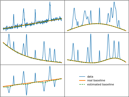
airpls (Adaptive Iteratively Reweighted Penalized Least Squares)

airpls() uses an exponential weighting of the negative residuals to attempt to provide a better fit than the asls method.

Minimized function:

\[\sum\limits_{i}^N w_i (y_i - z_i)^2 + \lambda \sum\limits_{i}^{N - d} (\Delta^d z_i)^2\]

Linear system:

\[(W + \lambda D_d^{\top} D_d) z = W y\]

Weighting:

\[\begin{split}w_i = \left\{\begin{array}{cr} 0 & y_i \ge z_i \\ exp{\left(\frac{t (y_i - z_i)}{|\mathbf{r}^-|}\right)} & y_i < z_i \end{array}\right.\end{split}\]

where \(t\) is the iteration number and \(|\mathbf{r}^-|\) is the l1-norm of the negative values in the residual vector \(\mathbf r\), ie. \(\sum\limits_{y_i - z_i < 0} |y_i - z_i|\).

(Source code, png)

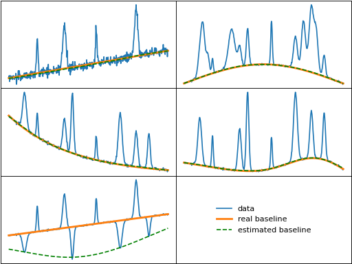
arpls (Asymmetrically Reweighted Penalized Least Squares)

arpls() uses a single weighting function that is designed to account for noisy data.

Minimized function:

\[\sum\limits_{i}^N w_i (y_i - z_i)^2 + \lambda \sum\limits_{i}^{N - d} (\Delta^d z_i)^2\]

Linear system:

\[(W + \lambda D_d^{\top} D_d) z = W y\]

Weighting:

\[w_i = \frac {1} {1 + exp{\left(\frac {2(r_i - (-\mu^- + 2 \sigma^-))} {\sigma^-} \right)}}\]

where \(r_i = y_i - z_i\) and \(\mu^-\) and \(\sigma^-\) are the mean and standard deviation, respectively, of the negative values in the residual vector \(\mathbf r\).

(Source code, png)

drpls (Doubly Reweighted Penalized Least Squares)

drpls() uses a single weighting function that is designed to account for noisy data, similar to arpls. Further, it takes into account both the first and second derivatives of the baseline and uses a parameter \(\eta\) to adjust the fit in peak versus non-peak regions.

Minimized function:

\[\sum\limits_{i}^N w_i (y_i - z_i)^2 + \lambda \sum\limits_{i}^{N - 2}(1 - \eta w_i) (\Delta^2 z_i)^2 + \sum\limits_{i}^{N - 1} (\Delta^1 (z_i))^2\]

where \(\eta\) is a value between 0 and 1 that controls the effective value of \(\lambda\).

Linear system:

\[(W + D_1^{\top} D_1 + \lambda (I - \eta W) D_2^{\top} D_2) z = W y\]

where \(I\) is the identity matrix.

Weighting:

\[w_i = \frac{1}{2}\left( 1 - \frac {exp(t)(r_i - (-\mu^- + 2 \sigma^-))/\sigma^-} {1 + abs[exp(t)(r_i - (-\mu^- + 2 \sigma^-))/\sigma^-]} \right)\]

where \(r_i = y_i - z_i\), \(t\) is the iteration number, and \(\mu^-\) and \(\sigma^-\) are the mean and standard deviation, respectively, of the negative values in the residual vector \(\mathbf r\).

(Source code, png)

iarpls (Improved Asymmetrically Reweighted Penalized Least Squares)

iarpls() is an attempt to improve the arpls method, which has a tendency to overestimate the baseline when fitting small peaks in noisy data, by using an adjusted weighting formula.

Minimized function:

\[\sum\limits_{i}^N w_i (y_i - z_i)^2 + \lambda \sum\limits_{i}^{N - d} (\Delta^d z_i)^2\]

Linear system:

\[(W + \lambda D_d^{\top} D_d) z = W y\]

Weighting:

\[w_i = \frac{1}{2}\left( 1 - \frac {exp(t)(r_i - 2 \sigma^-)/\sigma^-} {\sqrt{1 + [exp(t)(r_i - 2 \sigma^-)/\sigma^-]^2}} \right)\]

where \(r_i = y_i - z_i\), \(t\) is the iteration number, and \(\sigma^-\) is the standard deviation of the negative values in the residual vector \(\mathbf r\).

(Source code, png)

aspls (Adaptive Smoothness Penalized Least Squares)

aspls(), similar to the iarpls method, is an attempt to improve the arpls method, which it does by using an adjusted weighting function and an additional parameter \(\alpha\).

Minimized function:

\[\sum\limits_{i}^N w_i (y_i - z_i)^2 + \lambda \sum\limits_{i}^{N - d} \alpha_i (\Delta^d z_i)^2\]

where

\[\alpha_i = \frac {abs(r_i)} {max(abs(\mathbf r))}\]

Linear system:

\[(W + \lambda \alpha D_d^{\top} D_d) z = W y\]

Weighting:

\[w_i = \frac {1} {1 + exp{\left(\frac {0.5 (r_i - \sigma^-)} {\sigma^-} \right)}}\]

where \(r_i = y_i - z_i\) and \(\sigma^-\) is the standard deviation of the negative values in the residual vector \(\mathbf r\). (Note that the \(0.5 (r_i - \sigma^-) / \sigma^-\) term is different than the published version of the asPLS, which used \(2 (r_i - \sigma^-) / \sigma^-\). pybaselines uses the factor of 0.5 since it matches the results in Table 2 and Figure 5 of the asPLS paper closer than the factor of 2 and fits noisy data much better).

(Source code, png)

psalsa (Peaked Signal's Asymmetric Least Squares Algorithm)

psalsa() is an attempt at improving the asls method to better fit noisy data by using an exponential decaying weighting for positive residuals.

Minimized function:

\[\sum\limits_{i}^N w_i (y_i - z_i)^2 + \lambda \sum\limits_{i}^{N - d} (\Delta^d z_i)^2\]

Linear system:

\[(W + \lambda D_d^{\top} D_d) z = W y\]

Weighting:

\[\begin{split}w_i = \left\{\begin{array}{cr} p \cdot exp{\left(\frac{-(y_i - z_i)}{k}\right)} & y_i > z_i \\ 1 - p & y_i \le z_i \end{array}\right.\end{split}\]

where \(k\) is a factor that controls the exponential decay of the weights for baseline values greater than the data and should be approximately the height at which a value could be considered a peak.

(Source code, png)

derpsalsa (Derivative Peak-Screening Asymmetric Least Squares Algorithm)

derpsalsa() is an attempt at improving the asls method to better fit noisy data by using an exponential decaying weighting for positive residuals. Further, it calculates additional weights based on the first and second derivatives of the data.

Minimized function:

\[\sum\limits_{i}^N w_i (y_i - z_i)^2 + \lambda \sum\limits_{i}^{N - d} (\Delta^d z_i)^2\]

Linear system:

\[(W + \lambda D_d^{\top} D_d) z = W y\]

Weighting:

\[w_i = w_{0i} * w_{1i} * w_{2i}\]

where:

\[\begin{split}w_{0i} = \left\{\begin{array}{cr} p \cdot exp{\left(\frac{-[(y_i - z_i)/k]^2}{2}\right)} & y_i > z_i \\ 1 - p & y_i \le z_i \end{array}\right.\end{split}\]

\[w_{1i} = exp{\left(\frac{-[y_{sm_i}' / rms(y_{sm}')]^2}{2}\right)}\]

\[w_{2i} = exp{\left(\frac{-[y_{sm_i}'' / rms(y_{sm}'')]^2}{2}\right)}\]

\(k\) is a factor that controls the exponential decay of the weights for baseline values greater than the data and should be approximately the height at which a value could be considered a peak, \(y_{sm}'\) and \(y_{sm}''\) are the first and second derivatives, respectively, of the smoothed data, \(y_{sm}\), and \(rms()\) is the root-mean-square operator. \(w_1\) and \(w_2\) are precomputed, while \(w_0\) is updated each iteration.

(Source code, png)