Spline Baselines
Introduction
A spline is a piecewise joining of individual curves. There are different types of splines, but only basis splines (B-splines) will be discussed since they are predominantly used in pybaselines. B-splines can be expressed as:
where \(N\) is the number of points in \(x\), \(M\) is the number of spline basis functions, \(B_j(x_i)\) is the j-th basis function evaluated at \(x_i\), and \(c_j\) is the coefficient for the j-th basis (which is analogous to the height of the j-th basis). In pybaselines, the number of spline basis functions, \(M\), is calculated as the number of knots, num_knots, plus the spline degree minus 1.
For regular B-spline fitting, the spline coefficients that best fit the data are gotten from minimizing the least-squares:
where \(y_i\) and \(x_i\) are the measured data, and \(w_i\) is the weighting. In order to control the smoothness of the fitting spline, a penalty on the finite-difference between spline coefficients is added, resulting in penalized B-splines called P-splines (several good papers exist for an introduction to P-splines). The minimized function for P-splines is thus:
where \(\lambda\) is the penalty scale factor, and \(\Delta^d\) is the finite-difference operator of order d. Note that P-splines use uniformly spaced knots so that the finite-difference is easy to calculate.
The resulting linear equation for solving the above minimization is:
where \(W\) is the diagaonal matrix of the weights, \(B\) is the matrix containing all of the spline basis functions, and \(D_d\) is the matrix version of \(\Delta^d\) (same as explained for Whittaker-smoothing-based algorithms). P-splines have similarities with Whittaker smoothing; in fact, if the number of basis functions, \(M\), is set up to be equal to the number of data points, \(N\), and the spline degree is set to 0, then \(B\) becomes the identity matrix and the above equation becomes identical to the equation used for Whittaker smoothing.
Algorithms
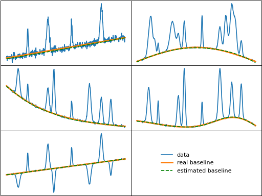
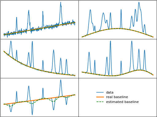
mixture_model (Mixture Model)
mixture_model() considers the data as a mixture model composed of
a baseline with noise and peaks. The weighting for the penalized spline fitting
the baseline is iteratively determined by fitting the residual with a normal
distribution centered at 0 (representing the noise), and a uniform distribution
for residuals >= 0 (and a third uniform distribution for residuals <= 0 if symmetric
is set to True) representing peaks. After fitting the total model to the residuals,
the weighting is calculated from the posterior probability for each value in the
residual belonging to the noise's normal distribution.

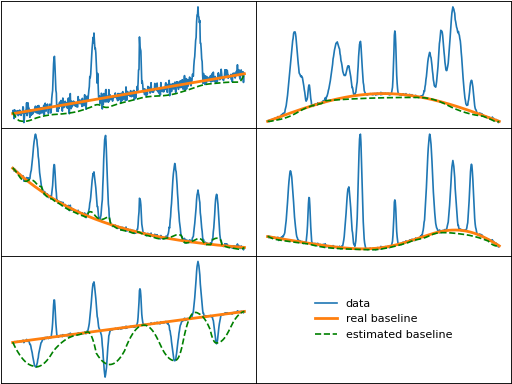
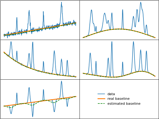
irsqr (Iterative Reweighted Spline Quantile Regression)
irsqr() uses penalized splines and iterative reweighted least squares
to perform quantile regression on the data.
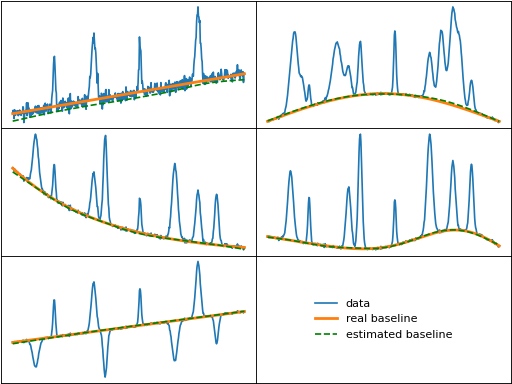
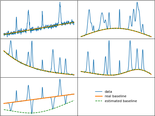
corner_cutting (Corner-Cutting Method)
corner_cutting() iteratively removes corner points and then creates
a quadratic Bezier spline from the remaining points. Continuity between
the individual Bezier curves is maintained by adding control points halfway
between all but the first and last non-corner points.
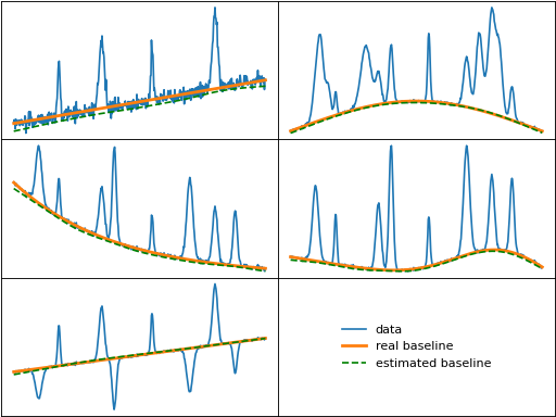
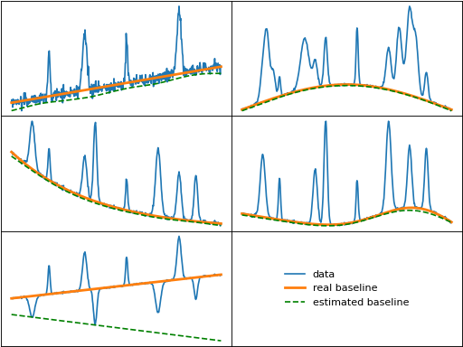
pspline_asls (Penalized Spline Version of asls)
pspline_asls() is a penalized spline version of asls().
Minimized function:
Linear system:
Weighting:
pspline_iasls (Penalized Spline Version of iasls)
pspline_iasls() is a penalized spline version of iasls().
Minimized function:
Linear system:
Weighting:
pspline_airpls (Penalized Spline Version of airpls)
pspline_airpls() is a penalized spline version of airpls().
Minimized function:
Linear system:
Weighting:
where \(t\) is the iteration number and \(|\mathbf{r}^-|\) is the l1-norm of the negative values in the residual vector \(\mathbf r\), ie. \(\sum\limits_{y_i - v_i < 0} |y_i - v_i|\). Note that the absolute value within the weighting was mistakenly omitted in the original publication, as specified by the author.

pspline_arpls (Penalized Spline Version of arpls)
pspline_arpls() is a penalized spline version of arpls().
Minimized function:
Linear system:
Weighting:
where \(r_i = y_i - v_i\) and \(\mu^-\) and \(\sigma^-\) are the mean and standard deviation, respectively, of the negative values in the residual vector \(\mathbf r\).

pspline_drpls (Penalized Spline Version of drpls)
pspline_drpls() is a penalized spline version of drpls().
Minimized function:
where \(\eta\) is a value between 0 and 1 that controls the effective value of \(\lambda\). \(w_{intp}\) are the weights, \(w\), after interpolating using \(x\) and the basis midpoints in order to map the weights from length \(N\) to length \(M\).
Linear system:
where \(I\) is the identity matrix.
Weighting:
where \(r_i = y_i - v_i\), \(t\) is the iteration number, and \(\mu^-\) and \(\sigma^-\) are the mean and standard deviation, respectively, of the negative values in the residual vector \(\mathbf r\).
pspline_iarpls (Penalized Spline Version of iarpls)
pspline_iarpls() is a penalized spline version of iarpls().
Minimized function:
Linear system:
Weighting:
where \(r_i = y_i - v_i\), \(t\) is the iteration number, and \(\sigma^-\) is the standard deviation of the negative values in the residual vector \(\mathbf r\).
pspline_aspls (Penalized Spline Version of aspls)
pspline_aspls() is a penalized spline version of aspls().
Minimized function:
where
and \(\alpha_{intp}\) is the \(\alpha\) array after interpolating using \(x\) and the basis midpoints in order to map \(\alpha\) from length \(N\) to length \(M\).
Linear system:
Weighting:
where \(r_i = y_i - v_i\), \(\sigma^-\) is the standard deviation of the negative values in the residual vector \(\mathbf r\), and \(k\) is the asymmetric coefficient (Note that the default value of \(k\) is 0.5 in pybaselines rather than 2 in the published version of the asPLS. pybaselines uses the factor of 0.5 since it matches the results in Table 2 and Figure 5 of the asPLS paper closer than the factor of 2 and fits noisy data much better).

pspline_psalsa (Penalized Spline Version of psalsa)
pspline_psalsa() is a penalized spline version of psalsa().
Minimized function:
Linear system:
Weighting:
where \(k\) is a factor that controls the exponential decay of the weights for baseline values greater than the data and should be approximately the height at which a value could be considered a peak.
pspline_derpsalsa (Penalized Spline Version of derpsalsa)
pspline_derpsalsa() is a penalized spline version of derpsalsa().
Minimized function:
Linear system:
Weighting:
where:
\(k\) is a factor that controls the exponential decay of the weights for baseline values greater than the data and should be approximately the height at which a value could be considered a peak, \(y_{sm}'\) and \(y_{sm}''\) are the first and second derivatives, respectively, of the smoothed data, \(y_{sm}\), and \(rms()\) is the root-mean-square operator. \(w_1\) and \(w_2\) are precomputed, while \(w_0\) is updated each iteration.
pspline_mpls (Penalized Spline Version of mpls)
pspline_mpls() is a penalized spline version of mpls().
Minimized function:
Linear system:
Weighting:
pspline_brpls (Penalized Spline Version of brpls)
pspline_brpls() is a penalized spline version of brpls().
Minimized function:
Linear system:
Weighting:
where:
\(r_i = y_i - v_i\), \(\beta\) is 1 minus the mean of the weights of the previous iteration, \(\sigma^-\) is the root mean square of the negative values in the residual vector \(\mathbf r\), and \(\mu^+\) is the mean of the positive values within \(\mathbf r\).
pspline_lsrpls (Penalized Spline Version of lsrpls)
pspline_lsrpls() is a penalized spline version of lsrpls().
Minimized function:
Linear system:
Weighting:
where \(r_i = y_i - v_i\), \(t\) is the iteration number, and \(\mu^-\) and \(\sigma^-\) are the mean and standard deviation, respectively, of the negative values in the residual vector \(\mathbf r\).
