Polynomial Baselines
Introduction
A polynomial can be expressed as
where \(\beta\) is the array of coefficients for the polynomial.
For regular polynomial fitting, the polynomial coefficients that best fit data are gotten from minimizing the least-squares:
where \(y_i\) and \(x_i\) are the measured data, \(p(x_i)\) is the polynomial estimate at \(x_i\), and \(w_i\) is the weighting.
However, since only the baseline of the data is desired, the least-squares approach must be modified. For polynomial-based algorithms, this is done by 1) only fitting the data in regions where there is only baseline (termed selective masking), 2) modifying the y-values being fit each iteration, termed thresholding, or 3) penalyzing outliers.
Selective Masking
Selective masking is the simplest of the techniques. There are two ways to use selective masking in pybaselines.
First, the input dataset can be trimmed/masked (easy to do with numpy) to not
include any peak regions, the masked data can be fit, and then the resulting
polynomial coefficients (must set return_coef to True) can be used to create
a polynomial that spans the entirety of the original dataset.
import numpy as np
import matplotlib.pyplot as plt
from pybaselines.utils import gaussian
from pybaselines import Baseline

x = np.linspace(1, 1000, 500)
signal = (
    gaussian(x, 6, 180, 5)
    + gaussian(x, 8, 350, 10)
    + gaussian(x, 15, 400, 8)
    + gaussian(x, 13, 700, 12)
    + gaussian(x, 9, 800, 10)
)
real_baseline = 5 + 15 * np.exp(-x / 400)
noise = np.random.default_rng(1).normal(0, 0.2, x.size)
y = signal + real_baseline + noise

# bitwise "or" (|) and "and" (&) operators for indexing numpy array
non_peaks = (
    (x < 150) | ((x > 210) & (x < 310))
    | ((x > 440) & (x < 650)) | (x > 840)
)
x_masked = x[non_peaks]
y_masked = y[non_peaks]

# fit only the masked x and y
_, params = Baseline(x_masked).poly(y_masked, poly_order=3, return_coef=True)
# recreate the polynomial using numpy and the full x-data
baseline = np.polynomial.Polynomial(params['coef'])(x)

# Alternatively, just use numpy:
# baseline = np.polynomial.Polynomial.fit(x_masked, y_masked, 3)(x)

fig, ax = plt.subplots(tight_layout={'pad': 0.2})
data_handle = ax.plot(y)
baseline_handle = ax.plot(baseline, '--')
masked_y = y.copy()
masked_y[~non_peaks] = np.nan
masked_handle = ax.plot(masked_y)
ax.set_yticks([])
ax.set_xticks([])
ax.legend(
    (data_handle[0], masked_handle[0], baseline_handle[0]),
    ('data', 'non-peak regions', 'fit baseline'), frameon=False
)
plt.show()

The second way is to keep the original data, and input a custom weight array into the fitting function with values equal to 0 in peak regions and 1 in baseline regions.
weights = np.zeros(len(y))
weights[non_peaks] = 1
# directly create baseline by inputting weights
baseline = Baseline(x).poly(y, poly_order=3, weights=weights)[0]

# Alternatively, just use numpy:
# baseline = np.polynomial.Polynomial.fit(x, y, 3, w=weights)(x)

fig, ax = plt.subplots(tight_layout={'pad': 0.2})
data_handle = ax.plot(y)
baseline_handle = ax.plot(baseline, '--')
masked_y = y.copy()
masked_y[~non_peaks] = np.nan
masked_handle = ax.plot(masked_y)
ax.set_yticks([])
ax.set_xticks([])
ax.legend(
    (data_handle[0], masked_handle[0], baseline_handle[0]),
    ('data', 'non-peak regions', 'fit baseline'), frameon=False
)
plt.show()

As seen above, both ways produce the same resulting baseline, but the second way (setting weights) is much easier and faster since the baseline is directly calculated.
The only algorithm in pybaselines that requires using selective masking is
poly(), which is normal polynomial least-squares fitting as described
above. However, all other polynomial techniques allow inputting custom weights
in order to get better fits or to reduce the number of iterations.
The use of selective masking is generally not encouraged since it is time consuming to select the peak and non-peak regions in each set of data, and can lead to hard to reproduce results.
Thresholding
Thresholding is an iterative method that first fits the data using traditional least-squares, and then sets the next iteration's fit data as the element-wise minimum between the current data and the current fit. The figure below illustrates the iterative thresholding.

The algorithms in pybaselines that use thresholding are modpoly(),
imodpoly(), and loess() (if use_threshold is True).
Penalyzing Outliers
The algorithms in pybaselines that penalyze outliers are
penalized_poly(), which incorporate the penalty directly into the
minimized cost function, and loess() (if use_threshold is False),
which incorporates penalties by applying lower weights to outliers. Refer
to the particular algorithms below for more details.
Algorithms
poly (Regular Polynomial)
poly() is simple least-squares polynomial fitting. Use selective
masking, as described above, in order to use it for baseline fitting.
Note that the plots below are just the least-squared polynomial fitting of the data since masking is time-consuming.

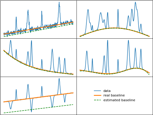
modpoly (Modified Polynomial)
modpoly() uses thresholding, as explained above, to iteratively fit a polynomial
baseline to data. modpoly is also sometimes called "ModPolyFit" in literature, and both
modpoly and imodpoly are sometimes referred to as "IPF" or "Iterative Polynomial Fit".
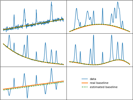
imodpoly (Improved Modified Polynomial)
imodpoly() is an attempt to improve the modpoly algorithm for noisy data,
by including the standard deviation of the residual (data - baseline) when performing
the thresholding. The number of standard deviations included in the thresholding can
be adjusted by setting num_std. imodpoly is also sometimes called "IModPolyFit" or "Vancouver Raman Algorithm" in literature,
and both modpoly and imodpoly are sometimes referred to as "IPF" or "Iterative Polynomial Fit".
Note
If using a num_std of 0, imodpoly may still produce different results than modpoly
due to their different exit criteria.
Note
Interesting historical note: an iterative masking-based polynomial method was proposed by Liu J., et al. in 1987 that based the mask each iteration on whether data points were one standard error above the calculated baseline (essentially a masked version of imodpoly 20 years before imodpoly was developed). However, it is much less stable than thresholding-based techniques like imodpoly since if the exit criteria is not properly set, few data points can remain for the polynomial fitting and cause severe misfitting of the baseline.
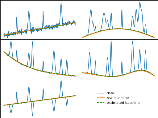
penalized_poly (Penalized Polynomial)
penalized_poly() (sometimes referred to as "backcor" in literature) fits a
polynomial baseline to data using non-quadratic cost functions. Compared to the quadratic
cost function used in typical least-squares as discussed above, non-quadratic cost funtions
allow outliers above a user-defined threshold to have less effect on the fit. pentalized_poly
has three different cost functions:
Huber
truncated-quadratic
Indec
In addition, each cost function can be either symmetric (to fit a baseline to data with both positive and negative peaks) or asymmetric (for data with only positive or negative peaks). The plots below show the symmetric and asymmetric forms of the cost functions.

loess (Locally Estimated Scatterplot Smoothing)
loess() (sometimes referred to as "rbe" or "robust baseline estimate" in literature)
is similar to traditional loess/lowess
but adapted for fitting the baseline. The baseline at each point is estimated by using
polynomial regression on the k-nearest neighbors of the point, and the effect of outliers
is reduced by iterative reweighting.
Note
Although not its intended use, the loess function can be used for smoothing like
"traditional loess", simply by settting symmetric_weights to True and scale to ~4.05.

quant_reg (Quantile Regression)
quant_reg() fits a polynomial to the baseline using quantile regression.

goldindec (Goldindec Method)
goldindec() fits a polynomial baseline to data using non-quadratic cost functions,
similar to penalized_poly(), except that it only allows asymmetric cost functions.
The optimal threshold value between quadratic and non-quadratic loss is iteratively optimized
based on the input peak_ratio value.
