Working with Masked or Missing Data

There are cases where data needs to be filtered/masked before processing, for example a faulty detector can result in problematic regions in measurements. In these cases, baseline correction on the raw data could lead to severely incorrect fits. One such use of masking in literature is presented by Temmink, et al. for removing downward spikes in mid-infrared data collected from the James Webb Space Telescope before performing baseline correction. This example will detail how to handle working with masked data for the various types of baseline correction algorithms in pybaselines.

As a preface for this guide, the author of this library acknowledges that masking could potentially be handled internally within each individual algorithm to make them "mask-aware". However, it would be a large change to the codebase, and there are many edge cases that would make it a non-trivial endeavor. Support for masking following the guidelines presented in this example could alternatively be added as an optimizer-type algorithm, but, in the author's opinion, making one single function that is expected to cover 60+ different algorithms would be fiddly at best and very prone to bugs. Therefore, this guide is presented as a starting point for users to adapt for targeting a spectific baseline correction algorithm or group of algorithms.

The various algorithms in pybaselines can be broadly grouped into three different categories for how they handle masked data:

1. Methods that directly support masking by inputting the mask as weights, which includes all classification and polynomial methods except for loess() and quant_reg(). They are not NaN-aware, however, so if working with missing data, that has to be accounted for.

2. Methods that do iterative reweighting, such as Whittaker smoothing methods, most spline methods, loess() and quant_reg(). As to be covered later in this guide, it is relatively easy to emulate a "mask-aware" implementation of these algorithms by making use of the output weights in the parameter dictionary to perform weighted interpolation in masked regions.

3. All other methods. Most would not be able to have a "mask-aware" version and would instead rely simply on interpolation of the input data, so whether this was handled internally or externally in user-code, the results would be the same.

import matplotlib.pyplot as plt
import numpy as np
from scipy.interpolate import PchipInterpolator

from pybaselines import Baseline
from pybaselines.utils import gaussian, relative_difference
from pybaselines._banded_utils import PenalizedSystem
from pybaselines._weighting import _arpls


x = np.linspace(500, 4000, 1000)
signal = (
    + gaussian(x, 8, 650, 16)
    + gaussian(x, 9, 1100, 50)
    + gaussian(x, 8, 1350, 20)
    + gaussian(x, 11, 2800, 20)
    + gaussian(x, 8, 2900, 20)
    + gaussian(x, 5, 3400, 40)
)
baseline = 0.08 + 0.00004 * (x - 1000) + gaussian(x, 10, 1900, 800)
rng = np.random.default_rng(123)
noise = rng.normal(0, 0.1, len(x))
y = signal + baseline + noise

baseline_fitter = Baseline(x)

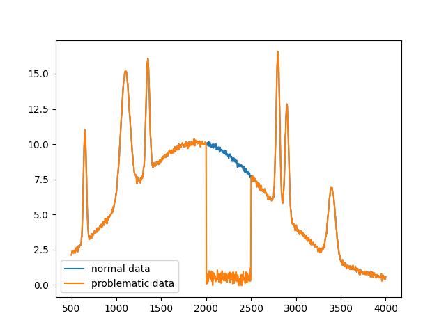
This example will emulate an issue with the detector such that a certain spectral region is just noise.

bad_region = (x > 2000) & (x < 2500)

y_bad = y.copy()
y_bad[bad_region] = rng.normal(0.5, 0.25, len(x[bad_region]))

plt.plot(x, y, label='normal data')
plt.plot(x, y_bad, label='problematic data')
plt.legend()

To start, the mask for fitting the data has to be made. This can be done by eye if fitting a few datasets, or can be automated using some metric. Many classification methods use different methods for excluding positive peaks; for excluding negative peaks, see Temmink, et al. for an example. This example will simply define the mask region by hand.

fit_mask = (x < 1900) | (x > 2550)  # 1 in regions to fit, 0 in masked region

First, the algorithms that are already mask-aware to a certain extent will be covered. For these algorithms, the mask needs to simply be input as weights, and any NaN values need to be replaced (with zeros, through interpolation, or using numpy.nan_to_num()).

non_masked_std_distributionc = baseline_fitter.std_distribution(
    y_bad, half_window=20, num_std=3
)[0]
masked_std_distribution = baseline_fitter.std_distribution(
    y_bad, half_window=20, num_std=3, weights=fit_mask
)[0]

non_masked_imodpoly = baseline_fitter.imodpoly(y_bad, poly_order=5, num_std=0.1)[0]
masked_imodpoly = baseline_fitter.imodpoly(y_bad, poly_order=5, num_std=0.1, weights=fit_mask)[0]

_, (ax1, ax2) = plt.subplots(2, layout='constrained')
ax1.set_title('std_distribution')
ax2.set_title('imodpoly')

ax1.plot(x, y_bad, label='data')
ax1.plot(x, non_masked_std_distributionc, label='non-masked baseline')
ax1.plot(x, masked_std_distribution, label='masked baseline')
ax1.legend()

ax2.plot(x, y_bad, label='data')
ax2.plot(x, non_masked_imodpoly, label='non-masked baseline')
ax2.plot(x, masked_imodpoly, label='masked baseline')
ax2.legend()

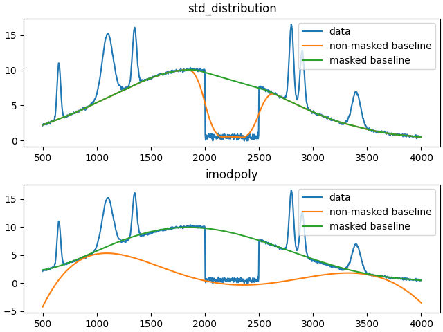
As seen in the plots above, the desired baselines can be obtained by simply inputting the mask as weights.

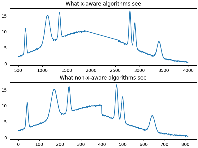
For all other non-mask-aware algorithms, interpolation is required for either the input data or the output baseline. It is generally recommended to interpolate the input data before passing the data to a baseline correction method rather than passing the masked data to the method and interpolating after since a large majority of algorithms are not x-aware, so the two regions on the edge of the mask would be assumed to be connected for those algorithms, as shown below, and would subsequently cause edge effects. Knowing which algorithms are x-aware and which are not is an implementation detail that is typically not apparent without intimate knowledge of each algorithm, so assuming all algorithms are not x-aware and interpolating before baseline correction is the safer route.

Note that as a generalization, polynomial, spline, and classifcation methods are x-aware while Whittaker, morphological, and smoothing methods are not.

_, (ax1, ax2) = plt.subplots(2, layout='constrained')
ax1.plot(x[fit_mask], y[fit_mask])
ax2.plot(y[fit_mask])
ax1.set_title('What x-aware algorithms see')
ax2.set_title('What non-x-aware algorithms see')

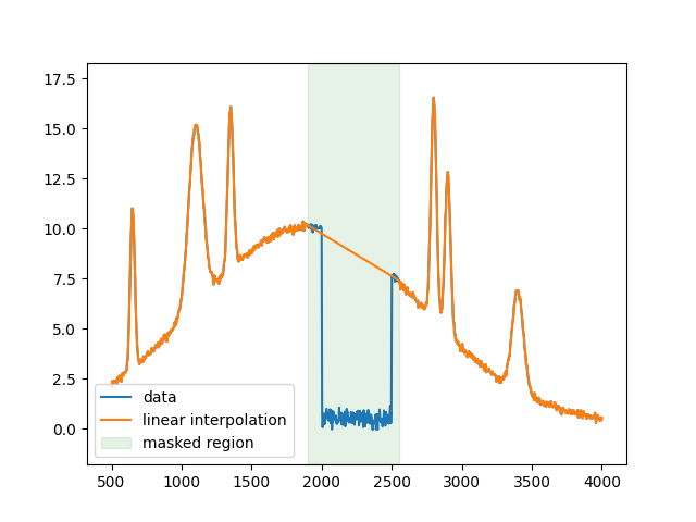
For the next example, simple linear interpolation will be used.

y_linear = np.interp(x, x[fit_mask], y_bad[fit_mask])
plt.figure()
plt.plot(x, y_bad, label='data')
plt.plot(x, y_linear, label='linear interpolation')
plt.fill_between(
    x[~fit_mask], 0, 1, color='green', alpha=0.1, transform=plt.gca().get_xaxis_transform(),
    label='masked region'
)
plt.legend()

Next are algorithms that use iterative reweighting. While the majority of these methods allow inputting weights, the input weights are just used for the first iteration to jump-start the calculation and are ignored in subsequent calculations. "Mask-aware" versions of these algorithms could be implemented, as shown below for the arPLS algorithm. However, the "mask-aware" behavior can be closely approximated simply by using weighted interpolation, to be shown below.

def masked_arpls(y, mask=None, lam=1e5, diff_order=2, tol=1e-3, max_iter=50, weights=None):
    """A mask-aware version of the arpls algorithm."""
    len_y = len(y)
    if mask is None:
        mask = np.ones(len_y, dtype=bool)
        y_fit = y
    else:
        y_fit = 1 * y  # don't want to override the input y, so make a copy
        y_fit[~mask] = 0  # cover that case of nan values in y since 0 * nan = nan rather than 0
    if weights is None:
        weights = np.ones(len_y)
    else:
        weights = 1 * weights  # don't want to override the input weights, so make a copy
    weights[~mask] = 0
    whittaker_system = PenalizedSystem(len(y), lam=lam, diff_order=diff_order)
    for _ in range(max_iter):
        baseline = whittaker_system.solve(
            whittaker_system.add_diagonal(weights), weights * y_fit,
        )
        # need to ignore the problem regions in y since they would otherwise affect
        # the arpls weighting; could alternatively do:
        # _arpls(np.interp(x, x[mask], y[mask]), baseline) to approximate
        # the y-values, but it leads to a slightly different result
        calc_weights, exit_early = _arpls(y[mask], baseline[mask])
        if exit_early:
            break
        new_weights = np.zeros(len_y)
        new_weights[mask] = calc_weights
        if relative_difference(weights, new_weights) < tol:
            break
        weights = new_weights

    return baseline

For iteratively reweighted algorithms, the best way to approximate a fully "mask-aware" version of the algorithms is to interpolate the input and get an approximated baseline. Then, the output weights in the region to be excluded should be set to 0, and the method should be called again for a single iteration, which can typically be done by setting the tolerance to infinity.

lam = 1e5
non_masked_arpls = baseline_fitter.arpls(y_bad, lam=lam)[0]
masked_arpls = masked_arpls(y_bad, mask=fit_mask, lam=lam)
initial_fit, params = baseline_fitter.arpls(y_linear, lam=lam)
params['weights'][~fit_mask] = 0
weighted_arpls = baseline_fitter.arpls(y_linear, lam=lam, weights=params['weights'], tol=np.inf)[0]

plt.figure()
plt.plot(x, y_bad)
plt.plot(x, non_masked_arpls, label='non-masked')
plt.plot(x, masked_arpls, label='mask-aware')
plt.plot(x, initial_fit, label='initial interpolated fit')
plt.plot(x, weighted_arpls, '--', label='final weighted interpolation')

plt.legend()

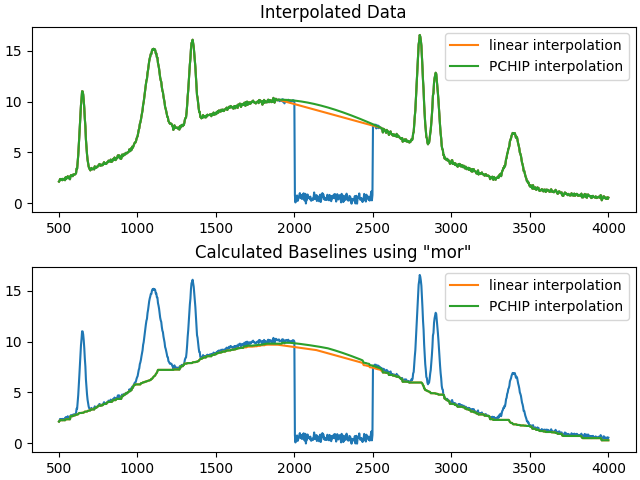
For all other algorithms, the performance is directly tied to the interpolation since information about the mask cannot be integrated into the method. For example, the difference between using linear interpolation and PCHIP interpolation is shown below.

y_pchip = PchipInterpolator(x[fit_mask], y[fit_mask])(x)
_, (ax1, ax2) = plt.subplots(2, layout='constrained')
ax1.set_title('Interpolated Data')
ax2.set_title('Calculated Baselines using "mor"')

ax1.plot(x, y_bad)
ax1.plot(x, y_linear, label='linear interpolation')
ax1.plot(x, y_pchip, label='PCHIP interpolation')
ax1.legend()

half_window = 35
mor_linear = baseline_fitter.mor(y_linear, half_window=half_window)[0]
mor_pchip = baseline_fitter.mor(y_pchip, half_window=half_window)[0]
ax2.plot(x, y_bad)
ax2.plot(x, mor_linear, label='linear interpolation')
ax2.plot(x, mor_pchip, label='PCHIP interpolation')
ax2.legend()

plt.show()